Algebraic geometry for the working programmer
Blog / Technical reports
In this series of posts, we investigate the duality between algebra and geometry in order to develop new types of lenses. In this first post, we review some basic ideas about algebraic geometry that will be needed in the coming posts.
$$
$$
1 Purpose
A traditional approach to algebraic geometry requires a course in commutative algebra, a great deal of patience for abstract nonsense, and then an innate love for elliptic curves. However, once one has scaled these imposing walls of what seems like pure math for its own sake, one finds a subject which has a great deal of algorithmic and philosophical merits.
Algebraic geometry is both the seed of the revolution in category theory developed by Grothendieck, and also is at the core of the algorithms in computer algebra that power systems like Mathematica, SAGE, or Macaulay2.
In this post, I aim to “pull back the curtain” on some of the things behind this wall of commutative algebra, and show why it is worth studying even if you don’t really care about elliptic curves or toric varieties or any of the other strange creatures that typically pull people into algebraic geometry from pure math. I will instead motivate the development of algebraic geometry from the perspective of someone trying to develop a symbolic algebra system.
There is also a point to all of this apart from pedagogy; this is a warmup for some new ideas for which a background in algebraic geometry is needed.
2 Expressions and evaluation
Computer algebra as generally construed is centered around the manipulation of syntactic expressions that are intended to represent mathematical formulas.
We might represent such an expression with a tree, where each node is either a function symbol, a variable, or a constant. For instance, the expression a^2 + 4b would be represented as:
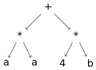
In a lisp, we would write down this tree as
In this notation, each matched pair of paretheses denotes a subtree, where the value at the root at the subtree is the first thing in the parentheses, called the head, and the rest of the parentheses denotes the subtrees attached to that root, called the arguments. We also allow numbers and symbols as arguments, which are the leaf nodes of the tree. We can express this in Julia with the following data structure.
Disclaimer: the code in this post will be optimized for brevity and clarity, not necessarily maintainability or usability. If you want to use the techniques in this post, there is a substantial amount of work to get something production-quality, including but not limited to parsing a nicer syntax and error-checking all computations.
Now, there are a great number of meaningless expressions that one can write down using the previous data structure. Generally, the first thing one would want to know about an expression is “does this make sense”? Of course, sense-making is relative. So the real question is “does this expression make sense relative to a certain signature”, and in order to answer that, we must define what a signature is. The rest of this section is based on a field of math called “universal algebra”, a good reference for which is Goguen (2021).
We say that an expression e is well-formed with respect to the signature (F, \mathrm{arity}) if the head of e is f \in F, e has \mathrm{arity}(f) arguments, and all of those arguments are also well-formed, or if e is just a symbol, representing a variable. The tree in Figure 1 is not well-formed with respect to F because there are numbers in it, however the left subtree is.
In order to deal with numbers, we add a nullary function symbol for every number.
With this signature, Figure 1 is well-formed.
One of the most natural things that one might want to do with an expression is evaluate it. However, we have allowed variables in our expressions; what does it mean to evaluate a variable? The answer is that we must talk about evaluating an expression in a context, which is an assignment of variables to values. But what is a value? One definition for a value would simply be a real number. But we can be more general than that.
We can evaluate an expression in any model, if we have an assignment of the variables in that expression to values in that model.
Evaluation is a recursive function, which is most naturally expressed with code.
abstract type Model{T} end

# Whenever we have a Model, we assume that we have a function of type
# interpret(m::Model{T}, f, args::Vector{T})::T

# evaluating a symbol just looks it up in the context
function evaluate(v::Symbol, ::Model{T}, ctx::Dict{Symbol, T}) where {T}
  ctx[v]
end
# evaluating an expression first evaluates the arguments, and then applies the
# interpretation of the head to those arguments
function evaluate(e::SymExpr, m::Model{T}, ctx::Dict{Symbol, T}) where {T}
  args = map(arg -> evaluate(arg, m, ctx), e.args)
  interpret(m, e.head, args)
end
struct MatrixModel <: Model{Matrix{Float64}}
  n::Int
end

# Here is the implementation of interpret for MatrixModel

function interpret(m::MatrixModel, f, args)
  if typeof(f) <: Number
    f * identity(m.n)
  elseif f == :+
    args[1] + args[2]
  elseif f == :*
    args[1] * args[2]
  end
end

evaluate(ex, MatrixModel(2), Dict(:a => [2. 0; 1 1], :b => [0 1.; 1. 0]))
# > 2×2 Matrix{Float64}:
# >   4.0  8.0
# >   11.0  1.0
We are now going to embark onto some category theory. But if you feel lost, know that the material that we are going to cover in the next sections is all just elaborations of the above 20 lines of code. If you understand what that code is doing, then just stare down the category theory until you can see that it’s doing the exact same thing.
We can get evaluation of expressions “for free” once we set up some categorical technology. We start by defining a category of models for a signature.
There is a functor U \colon \mathsf{Mdl}_F \to \mathsf{Set} that sends a model to its underlying set. This functor has a left adjoint \mathrm{Expr}_F \colon \mathsf{Set}\to \mathsf{Mdl}_F that sends a set X to the model \mathrm{Expr}_F(X) of F, where an element of \mathrm{Expr}_F(X) is a well-formed expression with respect to F with variables only from the set X.
The adjointness condition is that for any model M, maps X \to U(M) in \mathsf{Set} correspond bijectively to morphisms \mathrm{Expr}_F(X) \to M in \mathsf{Mdl}_F. A map c \colon X \to U(M) is what we called a context before; it assigns elements of X to values in M. Then the map c^{\ast} \colon \mathrm{Expr}_F(X) \to M simply sends an expression with free variables in X to its evaluation with context c.
Thus, evaluation is given by the adjoint transpose!
Now, whenever you have an adjunction there is a monad and comonad associated with it. In this case, we care about the monad, which is given by $T_F = U _F $. This monad takes a set X and returns the set of well-formed expressions T_F X.
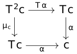
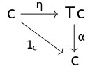
If (T,\eta,\mu) is a monad on a category \mathsf{C}, then a monad algebra1 of T consists of an element c \in \mathsf{C} and a morphism \alpha \colon T c \to c, such that the following diagrams commute
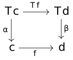
The algebras of T form a category \mathsf{Alg}_T, where a morphism from \alpha \colon T c \to c to \beta \colon T d \to d is a map f \colon c \to d such that the following commutes.
Whenever you have a monad T = UF coming from an adjunction F \colon \mathsf{C}\leftrightarrows \mathsf{D}\colon U, there is a functor from D to \mathsf{Alg}_T which sends d \in \mathsf{D} to the algebra U \mu \colon UFUd \to Ud, where \mu is the map given by applying the adjoint transpose to the identity U d \to U d.
In the case of our monad T_F = U \mathrm{Expr}_F, this says that for any model M there is a function U \mathrm{Expr}_F U M \to U M. That is, we can take an expression where the “variables” are elements of M, and evaluate that expression directly.
This gives another way of evaluating an expression with variables. We can take an expression e \in \mathrm{Expr}_F(X), then use functorality of \mathrm{Expr}_F to map c \colon X \to M across it and get an expression \mathrm{Expr}_F(c)(e) \in \mathrm{Expr}_F(M), and then evaluate this to get an element of M.
If we have an arbitrary T_F-algebra, then we can use a similar trick to evaluate expressions in a context as well. This implies that T_F-algebras are like models of F, and in fact this is exactly right! The functor from \mathsf{Mdl}_F to \mathsf{Alg}_{T_{F}} is an equivalence. M being a model of F is equivalent to being able to evaluate well-formed expressions with respect to F in M. This is because the monad algebra laws ensure that the algebra is determined solely by its action on the expressions which are non-recursive, i.e. which consist of a function symbol applied to values.
It turns out that there are general conditions under which this is true; that for an adjunction F \colon \mathsf{C}\rightleftarrows \mathsf{D}\colon U, \mathsf{D} is equivalent to the category of UF algebras; this is known as a monadicity theorem.
We’re now going to move on, and return to the computer algebra story. But the main takeaway that you should get from this section is that “models of a theory” and “algebras of a monad” are intimately connected; “models of a theory” tell you how to evaluate the function symbols, and “algebras of a monad” tell you how to evaluate arbitrary expressions, but the monad laws say that this evaluation is “generated” by just looking at the function symbols.
3 Symbolic functions
Now that we can evaluate expressions, the next thing one might want to do is construct functions using these expressions.
Suppose that one has an expression e in signature F with free variables contained in the set X, and that M is a model of F. Then given a context c \colon X \to M, or in other words, an element of M^X, we can evaluate e with context c to get an element of M.
Thus, there is a function from T_F(X) to M^X \to M for any model M. We can therefore think of an expression in variables x_1,\ldots,x_n as a “symbolic n-ary” operation.
But what if we want to consider functions M^X \to M^Y? This is the same as Y many maps M^x \to M. Thus, we need an expression in T_F(X) for every element of Y, i.e. a function Y \to T_F(X). It’s counterintuitive that the morphism is going in the opposite direction, but it comes directly from how we might write down such a function. I.e., if y = f(x), then \begin{align*} y_{1} &= f_{1}(x_{1},\ldots,x_{n}) \\ \vdots \\ y_{m} &= f_{m}(x_{1},\ldots,x_{m}) \end{align*}
Thus, the dual of the Kleisli category of T_F is the category of multivariate symbolic functions for a signature F. Let’s unpack that. The Kleisli category of T_F has as objects sets, and a morphism from Y to X is a function Y \to T_F(X). So the dual has as objects sets, and a morphism from X to Y is a function Y \to T_F(X). By what we showed earlier, for any model M of F, there is a functor from \operatorname{Kl}_{T_{F}}(\mathsf{Set})^{\mathrm{op}} to \mathsf{Set}, which sends f \colon Y \to T_F(X) to the map M^X \to M^Y given by evaluating each expression for each y \in Y with context c \in M^X.
Composition in this Kleisli category corresponds to substitution. I.e., if \begin{align*} y_{1} &= f_{1}(x_{1},\ldots,x_{n}) \\ \vdots \\ y_{m} &= f_{m}(x_{1},\ldots,x_{m}) \end{align*} and \begin{align*} z_{1} &= g_{1}(y_{1},\ldots,y_{m}) \\ \vdots \\ z_{k} &= g_{k}(y_{1},\ldots,y_{m}) \end{align*} then the composite is defined by \begin{align*} z_{1} &= g_{1}(f_{1}(x_{1},\ldots,x_{n}),\ldots,f_{m}(x_{1},\ldots,x_{n})) \\ \vdots \\ z_{k} &= g_{k}(f_{1}(x_{1},\ldots,x_{n}),\ldots,f_{m}(x_{1},\ldots,x_{n})) \end{align*} So, for instance, if F is the signature of \mathbb{R}-algebras, then there is a functor from \operatorname{Kl}_{T_{F}}(\mathsf{Set})^{\mathrm{op}} to \mathsf{Set}, which sends X to \mathbb{R}^X. This turns symbolic functions into real functions.
What are the advantages of working with symbolic functions instead of regular functions? Well, for one, they make it possible in the first place to work with functions at all! Ultimately, we are never working with “real functions” on a computer; we’re always working implicitly with symbolic functions.
Explicitly working with symbolic functions has other benefits however. Classically, one benefit is that we can compute the derivative of symbolic functions easily. Note that we can do this not just with polynomials; we can throw in function symbols \sin, \cos, \exp into our signature, and do all the exact same tricks as we’ve developed up until now! It might annoy algebraists, but who cares.
But the main benefit is that we might be able to find simpler representations of our functions, “canceling out” a large chunk of unnecessary computation so that our functions run faster in less memory.
In order to talk about this, however, we need to add laws to the picture.
Other examples of algebraic theories include the algebraic theories of groups and the algebraic theory of rings. Additionally, for any ring R, there is an algebraic theory of rings S along with maps R \to S, which is given by adding a nullary function symbol for every element of R, along with appropriate laws about how those elements add and multiply with each other.
A similar trick can be done to get an algebraic theory of modules over a ring R; take the theory of abelian groups, and then add a unary function symbol for every element of R representing scalar multiplication by that element. If R happens to be a field, then we get an algebraic theory of vector spaces. Note that there is no algebraic theory of fields, because multiplicative inverse is not defined on zero; but there is an algebraic theory of vector spaces, because we don’t need to worry about universally quantifying division; it is just implicit in how the unary function symbols interact.
The exact same story that we told for signatures can be told for theories. I.e., there is an adjunction between the category of models for a theory and \mathsf{Set}, and this adjunction induces a monad on \mathsf{Set}. The left adjoint sends a set X to the free model on that set. This is given by taking the model of the signature given by the well-formed expressions with variables taken from X, and then essentially just quotienting out until the laws hold. This models our ability to “rewrite” terms in a theory; the term (x + 1)(x + 1) can be rewritten to x^2 + 2x + 1. We might prefer the first one if we are trying to minimize multiplications, and the second one if we are trying to “normalize”.
In the case of \mathbb{R}-algebras, the free functor sends a set X to a \mathbb{R}-algebra which is easy to describe; it sends it to the \mathbb{R}-algebra \mathbb{R}[X] of polynomials with variables taken from X and coefficients in \mathbb{R}.
The canonical \mathbb{R}-algebra is just \mathbb{R}. Thus, we can think of a map Y \to \mathbb{R}[X] as a “symbolic” map from \mathbb{R}^X to \mathbb{R}^Y. In this particular case, it is just a polynomial map, but I say symbolic to emphasize that in the more general case when we aren’t talking about \mathbb{R}-algebras, we think about this as a symbolic map.
But by the adjunction, a map Y \to \mathbb{R}[X] is the same as a map \mathbb{R}[Y] \to \mathbb{R}[X]. We now arrive at the punchline of this section: maps of \mathbb{R}-algebras from \mathbb{R}[x_{1},\ldots,x_{n}] to \mathbb{R}[y_{1},\ldots,y_{m}] can be thought of as symbolic maps from \mathbb{R}^m to \mathbb{R}^n.
Thus, the dual of the category of free \mathbb{R}-algebras can be understood as the category of multivariate symbolic functions. We can see that this result should be interpreted more generally; the dual of the category of free models of an algebraic theory can be understood as a category of multivariate symbolic functions.
But why stop at free models? What about more general models? How might we interpret the dual of the category of algebraic theories as a category of “spaces and symbolic functions between them”? That is the subject of the next section.
4 Algebraic Spaces
In this section, we discuss symbolic functions between spaces which are more interesting than just \mathbb{R}^n. For the sake of concreteness, we will continue to work with \mathbb{R}-algebras, because these are more traditional than other algebraic theories, but a similar story could be told with other algebraic theories.
This is more traditional algebraic geometry material, and thus there are a wealth of references which cover similar material. For a classical algebraic geometry approach, the reader can refer to Eisenbud and Harris (2000), and a more modern approach relying more heavily on category theory can be found in Vakil (2017).
As a historical note, the definition of manifold in differential geometry used to be precisely zero sets of smooth functions.
Categorically speaking, a zero set of a function f \colon \mathbb{R}^n \to \mathbb{R}^k is given as the equalizer of the maps
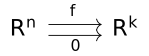
Recall that the equalizer is the universal object X with a map X \xrightarrow{i} \mathbb{R}^n such that f \circ i = 0 \circ i = 0. If we are working in a good category of spaces2, this is given precisely by the zero set of f, with appropriate structure.
Now, let’s compute this equalizer in our category of multivariate symbolic functions. A symbolic function f \colon \mathbb{R}^n \to \mathbb{R}^k is a \mathbb{R}-algebra homomorphism f \colon \mathbb{R}[y_1,\ldots,y_k] \to \mathbb{R}[x_1,\ldots,x_n]. We want to compute the “equalizer” of that function with the zero function (quiz: what is the zero function symbolically?). Because algebra is dual to geometry, this turns into computing the coequalizer in the category of free \mathbb{R}-algebras. But this category doesn’t have all coequalizers! Fortunately, there’s a convenient category hanging around that does have coequalizers: the category of all \mathbb{R}-algebras.
The coequalizer of f with 0 in the category of all \mathbb{R}-algebras is the quotient \mathbb{R}[x_1,\ldots,x_n]/(f(y_1),\ldots,f(y_n)) This is the set of polynomials in x_1,\ldots,x_n, “modded out” by the equivalence relation that p \sim q if there exist polynomials r_1,\ldots,r_n such that p = q + r_1 f(y_1) + \cdots + r_n f(y_n) Why does this make sense? Recall that f(y_i) is an expression in x_1,\ldots,x_n. When we assign values to the x_i such that f(y_i) = 0, then in fact, p evaluates to q. So if we are staying in the zero set of f, it makes sense to rewrite p to q.
In general, models of algebraic theories can always be expressed as quotients of free models. So this gives us an interpretation of the dual of the category of all models; it represents subspaces of product spaces, and symbolic functions between them.
We will finish with an observation. In a category with a terminal object 1, we think of maps 1 \to X as points of X. In the category of \mathbb{R}-algebras, there is an initial object, namely \mathbb{R}. So for a general \mathbb{R}-algebra S, we might think of maps S \to \mathbb{R} as “points” of S.
In the case of S = \mathbb{R}[x_1,\ldots,x_n], a map S \to \mathbb{R} is generated by where x_1,\ldots,x_n are sent. So such a map is precisely an element of \mathbb{R}^n. If we instead take S = \mathbb{R}[x_1,\ldots,x_n]/(p_1,\ldots,p_k), then a map S \to \mathbb{R} is again generated by where x_1,\ldots,x_k are sent. However, we also need to send p_1,\ldots,p_k to 0. So such a map is precisely an element v \in R^n, where p_1(v),\ldots,p_k(v) = 0. That is, it is an element of the zero set of p \colon \mathbb{R}^n \to \mathbb{R}^k. So the “points” of the “symbolic space” are just the points of the actual space!
The contravariant functor \operatorname{Hom}(-, \mathbb{R}) from the category of \mathbb{R}-algebras to \mathsf{Set} is called \mathrm{Spec}; it takes an \mathbb{R}-algebra to the “set of points” in the space that the \mathbb{R}-algebra represents. This functor is contravariant because (once more, say it with me) algebra is dual to geometry!