flowchart LR
  T("`**T**arget cells`") --> X[infection]
  V("`**V**irus`") --> X
  X --> I("`**I**nfected cells`")
  classDef transition fill:#53b6b2
  class X transition
Extending mass-action semantics, Part 1
Building a categorical model by hand
CatColab
modeling
Abstract
One particular use of formal categorical models is for exposition and learning. Indeed, the act of creating one can be a useful exercise for exposing implicit assumptions. In this post, we walk through the process of creating a diagrammatic representation of a system of ODEs and highlight the lessons learnt, as well as pointing towards why tools for formal modelling would be helpful.
Note
This post has a sequel: Part 2.
1 Some context
In January, Nina Fefferman, Mary Lou Zeeman, and myself, supported by the Center for Analysis and Prediction of Pandemic Expansion and the American Institute of Mathematics, organised a workshop:
We are in the process of preparing a report on the workshop, but, in short, “it was very good”, thanks entirely to the other organisers, the support of AIM, and the enthusiasm and expertise of the participants. However, this blog post is not about the workshop directly. Rather, I’d like to speak about a small piece of research that came out of a conversation during the workshop, and that has now landed in CatColab. I’d like to try to answer a few different questions in this post:
How can formal categorical modelling help people to better understand scientific models outside their expertise?
What do we mean when we say things like “categorical modelling can help make assumptions explicit”?
How can we allow for somewhat informal-looking diagrams to convey precise quantitative information?
While I won’t directly answer these questions, they’re in the background of the story that I’m going to tell. Then, in a future post, I’m going to focus more on the following:
How can software support the process of building categorical models?
What does it look like, in practice, to add new functionality to CatColab?
2 Understanding a model
I’m going to be talking about the model from the paper
A. Hoyer-Leitzel, S.M. Iams, A.J. Haslam-Hyde, M.L. Zeeman, N.H. Fefferman, “An immuno-epidemiological model for transient immune protection: A case study for viral respiratory infections”. Infectious Disease Modelling 8 (2023), pp. 855–864. DOI: 10.1016/j.idm.2023.07.004
which I’ll refer to as (Hoyer-Leitzel et al. 2023) or simply “the paper”.
2.1 The exercise
Let me start with the usual disclaimer: I am not an immuno-epidemiologist. In fact, I’m not even close, and have spent the last few months realising how little biology I actually know. But for the purpose of this exercise, this is actually a good thing because it gives an example of the kind of problem that I’m interested in studying: how can people sitting on opposite sides of a domain-specialist boundary better communicate? To be a bit more concrete, if I read a paper on a specific model in immuno-epidemiology and see some graph-like diagrams and systems of ordinary differential equations — things that I understand comparatively well — how can I be more sure that I’m not completely misinterpreting them? One of my preferred ways of teaching/learning is to flip things around and have the student explain things to the teacher, amongst other reasons because this often highlights key misunderstandings that can easily go unnoticed. I think the same thing can work well here:
Anyway, enough preamble. The model in the paper is almost given by the system of ODEs (Hoyer-Leitzel et al. 2023, Equation 1) \left\{ \begin{aligned} \dot{V} &= pI - cV - \mu VA - \beta VT \\\dot{T} &= gT\left( 1-\frac{T+I}{C_T} \right) - \beta' VT \\\dot{I} &= \beta' VT - \delta I - \kappa IF \\\dot{F} &= qI - dF \\\dot{B} &= m_1 V(1-B) - m_2 B \\\dot{A} &= m_3 B - rA - \mu' VA \end{aligned} \right. where the coefficients are described in the parameter table (Hoyer-Leitzel et al. 2023, Table 1), e.g. p is the “viral production rate”, c is the “viral clearance rate” , and so on. I say “almost” because I have omitted a smoothing term \frac{V}{V_m+V} that multiplies the three appearances of the VT monomial. The use of this smoothing term is actually one of the novel parts in the paper, and does raise a non-trivial question to the categorical modeller, but I’m going to save that story for another day.
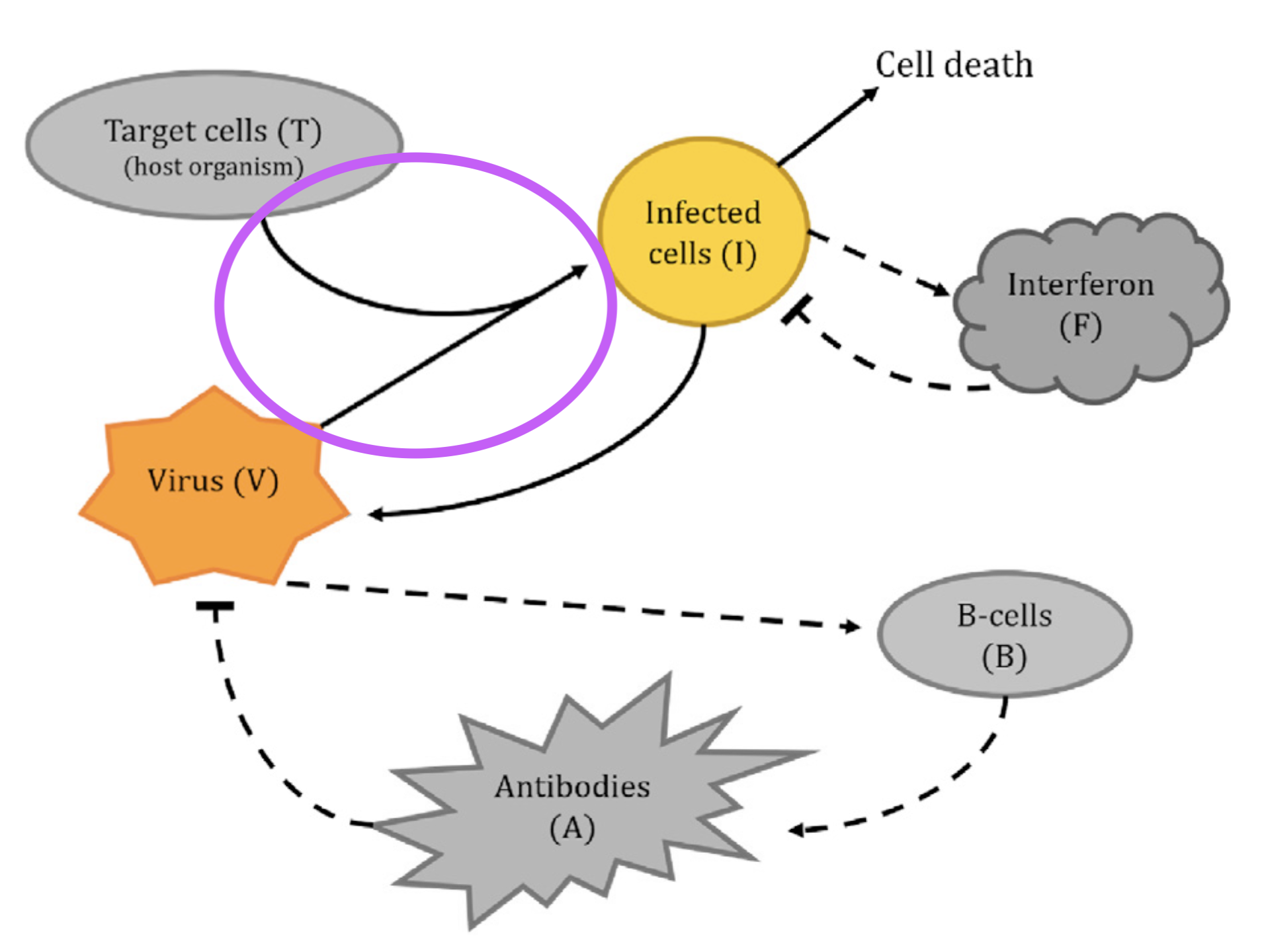
Alongside these quantitative parts, there’s a more high-level diagram (Hoyer-Leitzel et al. 2023, fig. 1) explaining the general processes described by the model, reproduced below.
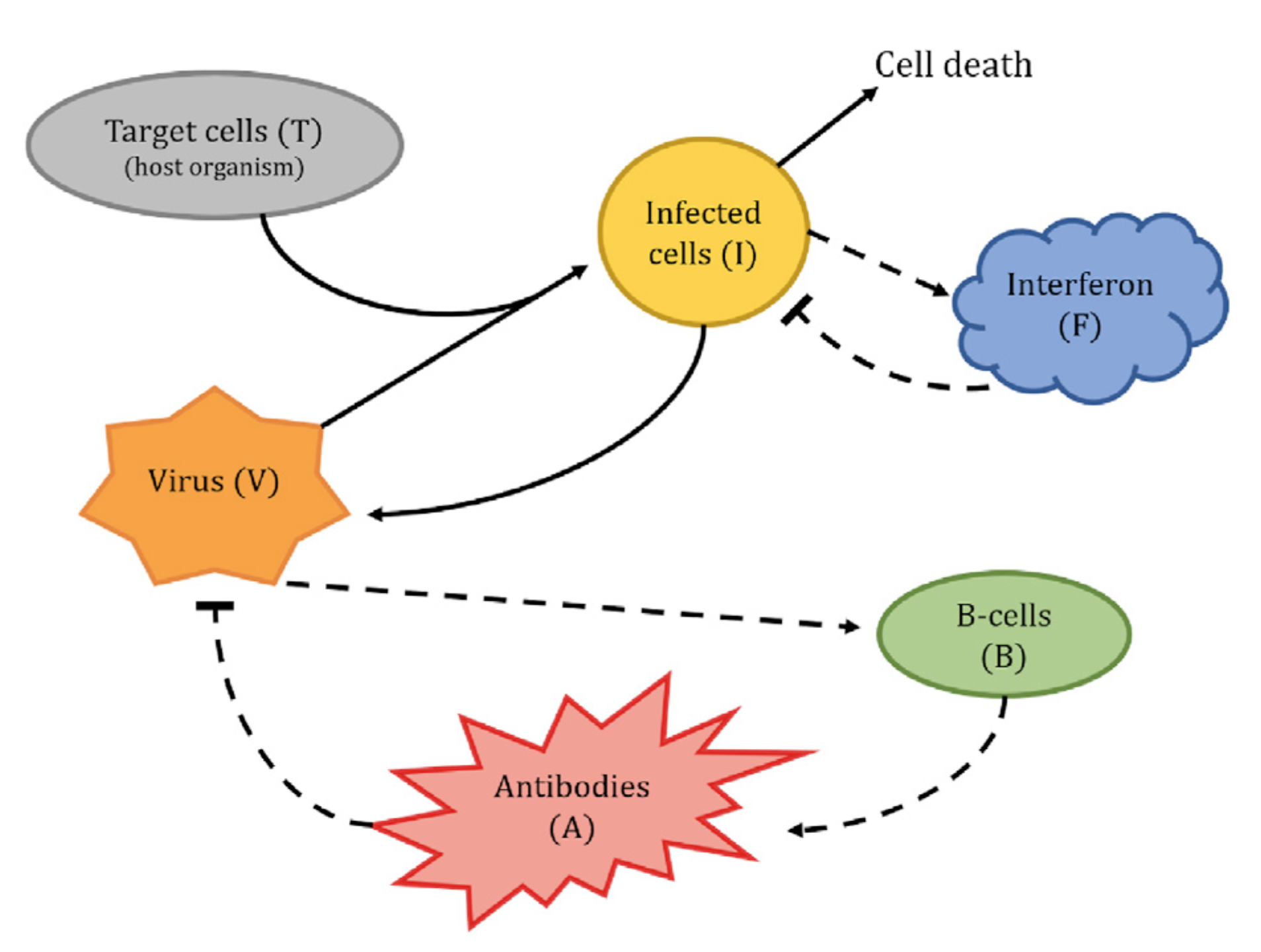
So here’s what we’re going to do: we’re going to draw our own version of the diagram, building it up bit by bit by grouping together terms in the system of ODEs, using the context given in the parameter table. What this will entail is “pairing up” terms in the ODEs to demarcate them as individual processes. The point is that we will likely not end up doing this in a biologically-correct way, but this method ensures that we have to make some specific choices and commit to these assumptions.
2.2 Rebuilding the model
Looking at the diagram, there’s some interaction between target cells T, the virus V, and the infected cells I. An educated guess tells me that viruses do something to target cells to turn them into infected cells and maybe get “used up” in the process, so this interaction will probably turn up in the equations for \dot{V}, \dot{T}, and \dot{I}. Having heard of mass-action dynamics from e.g. (Baez and Pollard 2017), I would guess that the corresponding terms in the ODEs will be proportional to the product of the inputs, i.e. VT. Putting this all together, it seems fair to assume that we have a correspondence between the circled part of the diagram and the boxed terms in the equations below:
\left\{ \begin{aligned} \dot{V} &= pI - cV - \mu VA - \boxed{\color{purple}\beta VT} \\\dot{T} &= gT\left( 1-\frac{T+I}{C_T} \right) - \boxed{\color{purple}\beta' VT} \\\dot{I} &= \boxed{\color{purple}\beta' VT} - \delta I - \kappa IF \\\dot{F} &= qI - dF \\\dot{B} &= m_1 V(1-B) - m_2 B \\\dot{A} &= m_3 B - rA - \mu' VA \end{aligned} \right.
Looking at the parameter table, we see that \beta and \beta' correspond to “rate of viral loss per target cell” and “rate of conversion from target cells to infected cells per virion”, respectively. This seems to confirm our conclusion, so let’s start drawing a diagram for ourselves.
2.2.1 The first interaction: infection
Rather than drawing multi-arrows (arrows with multiple inputs), we’ll take inspiration from Petri net notation and make interactions first-class elements, drawing them as boxes. Then our variables can be inputs or outputs of interactions. For example, we would draw this “infection” interaction like so:
This is intended to be read in a similar way to mass-action dynamics for Petri nets: each variable will have an ODE describing its behaviour, and each transition generates contributions (i.e. terms) of these ODEs. Whenever you see a transition, you should look at all the input variables (here, V and T) and take their product (VT). You then add this as a negative term to each of the ODEs corresponding to an input variable, and as a positive term to those corresponding to an output variable. So here we would get \left\{ \begin{aligned} \dot{V} &\overset{+}{=} VT \\\dot{T} &\overset{+}{=} VT \\\dot{I} &\overset{-}{=} VT \end{aligned} \right.
But the thing we’re going to do differently here is to also labelled the arrows with some data, namely \beta and \beta', corresponding to the coefficient of the monomial in the ODE. This should be interpreted as telling us the rate coefficient for that term. All in all then, we have a convention for (a) drawing diagrams, and (b) turning them into systems of ODEs.
flowchart LR
  T("`**T**arget cells`") -->|𝛽'| X[infection]
  V("`**V**irus`") -->|𝛽| X
  X -->|𝛽'| I("`**I**nfected cells`")
  classDef transition fill:#53b6b2
  class X transition
\leftrightsquigarrow \left\{ \begin{aligned} \dot{V} &\overset{+}{=} \beta VT \\\dot{T} &\overset{+}{=} \beta'VT \\\dot{I} &\overset{-}{=} \beta'VT \end{aligned} \right.
2.2.2 Different diagrams, clouds, and no links
Let’s move on to another interaction. Looking at the system of ODEs and the parameter table, it seems like the terms \left\{ \begin{aligned} \dot{V} &\overset{-}{=} \mu VA \\\dot{A} &\overset{-}{=} \mu'VA \end{aligned} \right. can also be paired up, coming from a virion/antibody interaction. We can add this to our diagram:
flowchart LR
  T("`**T**arget cells`") -->|𝛽'| X[infection]
  V("`**V**irus`") -->|𝛽| X
  X -->|𝛽'| I("`**I**nfected cells`")
  V -->|𝜇| Y{{antibody-virion binding}}
  A("`**A**ntibodies`") -->|𝜇'| Y
  classDef transition fill:#53b6b2
  classDef death fill:#ddd,color:#555
  class X transition
  class Y death
We haven’t drawn any output for this new interaction, but that’s because it concerns a quantity that we’ve decided we’re not interested in measuring, namely the number of “dead” viruses and/or antibodies. We could take inspiration from stock-flow/system structure diagrams and draw clouds to represent such quantities, but for the sake of simplicity we’re not going to do that and instead just make the interaction itself grey and hexagonal.
Anyway, adding this second interaction is an important step, because now our diagram really does look different from the one in (Hoyer-Leitzel et al. 2023). The latter shows antibodies as inhibiting virus production, whereas ours shows antibodies and viruses interacting in some process as sort of “equal players”. Maybe we could enrich our diagrams to allow for some sort of inhibition arrows, building up some sort of multi-ary stock-flow with links syntax. But I’m not going to do that right now, for a few reasons, but primarily because I don’t have the biological intuition to know what is correct. This is one example of what I meant by question (2) right at the start of this post: what does it mean to make our assumptions explicit? Here I’m showing that, to me, the antibody response interaction is of the same sort of shape/flavour/vibe as the infection interaction: it takes inputs and gives outputs, and the interaction itself is not modulated by some any parameter, or affected by any other variables. By building this diagram we are expressing our understanding of what we intend the model to represent, by essentially saying things like “I don’t believe in modulated/parametrised interactions, only direct agent-to-agent interactions”. Whether or not this is a good assumption is something to be discussed, but what I’m trying to point out here is that in order to do so we first need to make clear that we are indeed asserting this as an assumption.
We’re immediately going to see another example of this same phenomenon once we look at the equation governing \dot{F}. Interferons are named as such because they “interfere” with virus production (so Wikipedia tells me). In this model, it seems like they do so only by means of reducing the number of infected cells as \dot{I}\overset{-}{=}\kappa IF since there is no contribution to \dot{V} that directly involves the quantity F. Furthermore, the equation governing F is \dot{F} = qI - dF where q is the interferon production rate and d is the interferon degradation rate. To me, it sounds like neither of these terms are anything to do with the interferon-infected cell interaction term \dot{I}\overset{-}{=}\kappa IF, but I could very well be wrong. Either way, let’s commit my guess to our diagram:
flowchart LR
  I("`**I**nfected cells`")
  F("`Inter**f**erons`")
  X{{I-F interaction}}
  Y[interferon production]
  Z{{interferon degradation}}
  I -->|𝜅| X
  F -->|0| X
  I -->|0| Y
  Y -->|𝑞| F
  F -->|𝑑| Z
  classDef transition fill:#53b6b2
  classDef death fill:#ddd,color:#555
  class X death
  class Y transition
  class Z death
As a convenient shorthand, rather than labelling an arrow with a 0, from now on I’ll just draw a dotted arrow with no label. In particular, for example, our diagram now says that interferons do not get “used up” in the interferon-infected cell interaction.
We are led to consider the important question: what is the difference between an interaction that takes some input X but doesn’t “consume” it, and an interaction that does not take X as an input but instead accepts it as a parameter to modulate its rate? Again, we are making explicit in this model one of my assumptions:
2.2.3 Merging or separating interactions
Looking back at the system of ODEs, there are three terms given by the monomial I, namely \begin{aligned} \dot{V} &\overset{+}{=} pI \\\dot{I} &\overset{-}{=} \delta I \\\dot{F} &\overset{+}{=} qI. \end{aligned} Without looking up what the parameters p, \delta, and q mean, and just thinking about these as abstract ODEs, with no real context, there are multiple ways that we could build a diagram to recover them:
- There is a single interaction giving rise to all three monomial contributions
flowchart LR
  V("`**V**irus`")
  I("`**I**nfected cells`")
  F("`Inter**f**erons`")
  X[1]
  I -->|𝛿| X
  X -->|𝑝| V
  X -->|𝑞| F
  classDef transition fill:#53b6b2
  class X transition
- There are two interactions, with e.g. one pairing up the (+pI,+qI) terms and the other contributing just the -\delta I term
(or either of the two other possible pairings: (+pI,-\delta I) and +qI, or (+qI,-\delta I) and +pI)
flowchart LR
  V("`**V**irus`")
  I("`**I**nfected cells`")
  F("`Inter**f**erons`")
  X{{2a}}
  Y[2b]
  I -->|𝛿| X
  I -.-> Y
  Y -->|𝑝| F
  Y -->|𝑞| V
  classDef transition fill:#53b6b2
  classDef death fill:#ddd,color:#555
  class X death
  class Y transition
- There are three interactions, with each one contributing a single monomial term
flowchart LR
  V("`**V**irus`")
  I("`**I**nfected cells`")
  F("`Inter**f**erons`")
  X{{3a}}
  Y[3b]
  Z[3c]
  I -->|𝛿| X
  I -.-> Y
  I -.-> Z
  Y -->|𝑝| F
  Z -->|𝑞| V
  classDef transition fill:#53b6b2
  classDef death fill:#ddd,color:#555
  class X death
  class Y transition
  class Z transition
Although all three of these options describe exactly the same quantitative information (i.e the same system of ODEs), they clearly suggest different contextual information, namely “what are the actually interactions that are happening?”. The first and third option are at opposite ends of the spectrum, saying that everything all happens together or that everything all happens completely independently. Yet again, I do not have the biological intuition to know which one is correct, but, yet again, building this diagram rather than merely giving the ODEs means that I have to commit to one of them as an explicit assumption.
Reading the parameter table, we see that p is the viral production rate, q is the interferon production rate, and \delta is the death/removal rate of infected cells. Unfortunately, I can’t tell from this which option from the above is the best representation. But since we’ve already accounted for the interferon-infected cell interference in the \dot{I}\overset{-}{=}\kappa IF term, I’m going to go ahead and pick option 3, saying that these three interactions are all relatively independent of one another.
At this point, it might seem like what we’re doing is entirely the opposite of building some flexible model that will be useful for collaboration. We keep having to lock in assumptions and make choices and commit to them, and we’re not allowed any wriggle room. But this isn’t true.
Right now we’re building a single diagram (or a single model, if you like), and we’re (somewhat secretly) using category theory to do so: there are boxes and arrows between them. But category theory also lets us step back, zoom out, and do all the same tricks one dimension higher. What that means here is that we can think of this diagram itself as an object, and then ask what a morphism between such objects should be. For example, a morphism between diagrams could consists of an assignment of variable boxes (the green ones) to variable boxes, and collections/sequences of interaction boxes (the blue ones) to interaction boxes. This post is not the place to spell out the details, but we can give an example of this example: there should be a morphism from option 3 to option 2, given by “gluing together” interactions 3b and 3c into the single interaction 2b.
flowchart LR
  subgraph source
    direction LR
    I1("`**I**nfected cells`")
    V1("`**V**irus`")
    F1("`Inter**f**erons`")
    X1{{3a}}
    Y1[3b]
    Z1[3c]
    I1 -->|𝛿| X1
    I1 -.-> Y1
    I1 -.-> Z1
    Y1 -->|𝑝| F1
    Z1 -->|𝑞| V1
  end
  subgraph target
    direction LR
    V2("`**V**irus`")
    I2("`**I**nfected cells`")
    F2("`Inter**f**erons`")
    X2{{2a}}
    Y2[2b]
    I2 -->|𝛿| X2
    I2 -.-> Y2
    Y2 -->|𝑝| F2
    Y2 -->|𝑞| V2
  end
  source -->|morphism| target
  classDef transition fill:#53b6b2
  classDef death fill:#ddd,color:#555
  class X1 death
  class Y1 transition
  class Z1 transition
  class X2 death
  class Y2 transition
  classDef box fill:#fff,stroke:#555
  class source box
  class target box
2.2.4 The importance of brackets
This post is getting quite long, so here I’m just going to point out a problem for us to revisit in the future.
When solving ODEs, we are allowed to factor and expand out brackets as much as we want. Of course, mathematics say we can! For example, consider the two ODEs below: \dot{B} = m_1V(1-B) \tag{$\dagger$} \dot{B} = m_1V - m_1VB \tag{$\ddagger$} Of course, by simply expanding out the right-hand side of (\dagger), or factoring the right-hand side of (\ddagger), we can see that these equations are identical in terms of their solutions. But the key phrase is “in terms of their solutions”. Looking back at the original system of ODEs, note that there are many terms that could be factored but which have not been factored, e.g. in the equation for \dot{V} we have cV+\mu VA instead of V(c+\mu A), so why specifically write \dot{B}\overset{+}{=}m_1V(1-B)? Well, let’s consider how we would draw diagrams for (\dagger) and (\ddagger).
flowchart TB
  subgraph dagger ["Diagram (†)"]
    direction LR
    V("`**V**irus`")
    B("`**B**-cells`")
    X[X]
    V -.-> X
    X -->|"𝑚₁(1-𝐵)"| B
  end
  classDef transition fill:#53b6b2
  class X transition
  classDef box fill:#fff,stroke:#555
  class dagger box
flowchart TB
  subgraph ddagger ["Diagram (‡)"]
    direction LR
    V("`**V**irus`")
    B("`**B**-cells`")
    X[X]
    Y[Y]
    V -.-> X
    X -->|𝑚₁| B
    V -.-> Y
    B -->|𝑚₁| Y
  end
  classDef transition fill:#53b6b2
  class X transition
  class Y transition
  classDef box fill:#fff,stroke:#555
  class ddagger box
We can now see that there is a different problem with each of these diagrams:
In Diagram (†) we are cheating the mathematics.
We label an arrow with m_1(1-B), which is not a fixed real-valued parameter but rather a time-varying parameter that depends on the state variable B. This means that our formal mathematical story is no longer honest and our diagrams return to being mere pictures on a page.
In Diagram (‡) we are misconstruing the original system of ODEs.
It makes sense to read the single term contribution \dot{B}\overset{+}{=}m_1V(1-B) as saying that B grows relative to V with factor m_1 but in a self-regulating way that slowly turns off this process as B grows from 0 to 1. But in the diagram there are two separate processes, and it doesn’t suggest that one is modulating the other, merely that they might happen to cancel out.
The first problem is semi-fixable, but I definitely cannot claim to have a complete answer. It’s relatively straightforward to allow for a more expressive labelling of the arrows, but this problem of state variables themselves appearing in the parameters requires more thought.
The second problem is a bit more amenable to the tools in our current toolkit. What we are noticing is the following:
We could consider trying to change our made-up rules to amend this, but we have another option. Imagine taking the diagram and drawing a box around the two interactions:
flowchart LR
  V("`**V**irus`")
  subgraph boxed ["V–B interaction"]
    X[X]
    Y[Y]
  end
  B("`**B**-cells`")
  V -.-> X
  X -->|𝑚₁| B
  V -.-> Y
  B -->|𝑚₁| Y
  classDef transition fill:#53b6b2
  class X transition
  class Y transition
  classDef box fill:#fff,stroke:#555
  class boxed box
Now we take that box and close the lid, black-boxing what’s inside of it, and just labelling it with a big “V–B interaction” sticker:
flowchart LR
  V("`**V**irus`")
  T["V–B interaction"]
  B("`**B**-cells`")
  V -.-> T
  T --> B
  B --> T
  classDef boxed-transition fill:#53b6b2
  class T boxed-transition
As for what this means mathematically — how we update the rules to our formalism — this is again a story that deserves a bit more time to be properly told. Note that we also need to figure out how to label the arrows between the interaction box and B, since if we just label them both with m_1 then we won’t recover the correct equations.
To wrap up this current blog post we’re just going to cheat a bit, doing the same trick as in Diagram (†).
2.2.5 Our final diagram
We’ve pointed out essentially all of the complications and considerations of drawing a diagram for this specific system of ODEs. We should really talk more about the growth term gT(1-(T+1)/C_T) for T, but it’s somewhat related to the problems of the m_1V(1-B) term we just discussed, so I’m going to just mark both of them with a ⚠️ symbol for now.
All in all, we can write everything down in one big diagram:
flowchart TB
  T("`**T**arget cells`")
  V("`**V**irus`")
  I("`**I**nfected cells`")
  F("`Inter**f**erons`")
  A("`**A**ntibodies`")
  B("`**B**-cells`")
  X0[⚠️ target-cell growth ⚠️]
  X1[infection]
  X2{{interferon interference}}
  X3[virus production]
  X4[interferon production]
  Z3{{F death}}
  Y1[B-cell activation]
  Y2[antibody response]
  Y3[antibody-virion binding]
  Z1{{V death}}
  Z2{{I death}}
  Z4{{A death}}
  Z5{{B death}}
  T --> X0
  I --> X0
  X0 --> T
  T -->|𝛽'| X1
  V -->|𝛽| X1
  X1 -->|𝛽'| I
  I -->|𝜅| X2
  F -.-> X2
  I -.-> X3
  X3 -->|𝑝| V
  I -.-> X4
  X4 -->|𝑞| F
  V -.-> Y1
  Y1 -->|"⚠️ 𝑚₁(1-𝐵) ⚠️"| B
  B -.-> Y2
  Y2 -->|𝑚₃| A
  V -->|𝜇| Y3
  A -->|𝜇'| Y3
  V -->|𝑐| Z1
  I -->|𝛿| Z2
  F -->|𝑑| Z3
  A -->|𝑟| Z4
  B -->|𝑚₂| Z5
  classDef transition fill:#53b6b2
  classDef death fill:#ddd,color:#555
  class X0 transition
  class X1 transition
  class X2 death
  class X3 transition
  class X4 transition
  class Y1 transition
  class Y2 transition
  class Y3 transition
  class Z1 death
  class Z2 death
  class Z3 death
  class Z4 death
  class Z5 death
… so why does this blog post have a sequel?
3 Problems
Writing this blog post took a very long time, and part of the reason for that is how many mistakes I kept on making. The diagrams here are written in Mermaid, which I typed by hand. I’ve included the code for the final diagram below, so you can see what it looks like.
The mistakes I kept on making in writing this post were essentially all of the following form:
- I write down the equations generated by a part of the diagram and then realise that I’ve drawn an arrow between the wrong boxes, or in the wrong direction, or gotten two parameter labels swapped around, or …
- I count the number of interaction boxes and the number of monomial terms and see they don’t match up, and realise that I’ve missed a term
- I realise that I’ve just made a typo and this has lead to two things being swapped around, or a box called “inteferon” being created alongside one called “interferon”
- I make some mistake in the Mermaid code that means it won’t render
Since I was trying to recover a specific system of ODEs, my constant test was “take the diagram, turn it back into equations, and compare it to the original”. This helped me spot the above mistakes, but is itself vulnerable to a meta-mistake (which I also made many times), namely:
Fixing this last problem would dramatically improve my ability to fix all the other problems, and this is precisely the type of problem that sounds like something computers should be good at doing. In fact, I think that all of the types of problems that I’ve pointed out here are things that computers are good at helping us to avoid. Some of the simpler problems (mistakes in the Mermaid code, and typos in names of boxes) are solved by using a structure editor rather than a text editor.
Hey, what do you know — CatColab is a structure editor! But although it has an analysis for mass-action dynamics for Petri nets (and what we’ve been drawing are essentially Petri nets), it doesn’t support this variation where we give different rate coefficients for each input and output place of each transition; in CatColab, you can only give a rate coefficient for each transition.
However, the CatColab codebase is now mature and modular enough that this is not a problem. After some conversation with Evan and Jason, I spent a week implementing this feature so that I could repeat the above model-building exercise directly in CatColab. In the sequel to this blog post, I’m going to talk a bit about the actual development process, the changes we had to make, and how things now look in CatColab.
References
Baez, John C., and Blake S. Pollard. 2017. “A Compositional Framework for Reaction Networks.” Rev. Math. Phys. 29. https://doi.org/10.1142/S0129055X17500283.
Hoyer-Leitzel, A., S. M. Iams, A. J. Haslam-Hype, M. L. Zeeman, and N. H. Fefferman. 2023. “An Immuno-Epidemiological Model for Transient Immune Protection: A Case Study for Viral Respiratory Infections.” Infectious Disease Modelling 8: 855–64. https://doi.org/10.1016/j.idm.2023.07.004.