A Type Theory for Virtual Double Theories
Blog / Technical reports
A virtual double theory compactly specifies the shape of a categorical logic, which are used by CatColab to bestow models with types. These theories themselves can be described using a type theory for virtual double categories; in this post I will outline my (ongoing) work to refine this type theory and develop a corresponding semantic model and software implementation in the form of a small domain-specific language.
In many fields of mathematics, one is interested in studying the models of a particular theory: a first course on abstract algebra may consist of a survey of models for the theory of groups, and perhaps also for the theory of rings, while a student of computer science may be more interested in models of the theory of graphs. Broadly speaking, a theory determines the “shape” of a structure, consisting of a signature (a collection of generating symbols), which defines those structures’ “interface,” and axioms (equations or formulae), which describe this interface’s internal interactions and behavior.
Consider, for instance, the theory of monoids. One presentation for this theory might include symbols e and m representing the identity element and multiplication (respectively), together with axioms which make m associative and unital with respect to e. A model of this theory, that is, a concrete interpretation of the symbols of the theory as a set X with a nullary operation (i.e. a constant) e_X and a binary operation m_X satisfying these axioms, is then precisely the data of a monoid.
In the setting of categorical logic, we are interested in viewing theories themselves as categorical structures, rather than mere collections of symbols and equations relating them. We are particularly interested in the case when our theories are double categories, whose models are naturally valued in categories [1]. Such double theories can be presented by generators for their objects, morphisms, proarrows, and cells, along with axioms that introduce additional equalities between them. A model for a double theory consists of a (double) functorial1 interpretation of each of the theory’s generating symbols which respects the equalities imposed by the axioms.
Every double theory defines a corresponding domain-specific categorical logic. The double category encoding the interface of a monoidal category, for example, gives rise to the internal logic of monoidal categories. Although monoidal categories are fairly sophisticated pieces of machinery, the theory itself (as a double category) is quite simple, and can be presented with only a few generating symbols. Much like the (first-order) theory of monoids, the theory of monoidal categories must also be equipped with axioms that enforce the usual associativity and unitality of the monoidal product. A vast range of rich categorical structures can be seen as models of double theories which are easy to present with finite data, making them a convenient tool for embedding categorical logics in software.
CatColab, a collaborative modeling environment built on a foundation of category theory, is one such system, consisting of a gestalt of specialized sub-components for working with various domain-specific categorical logics [3,4]. One component that is currently missing from CatColab, however, is a language to specify the double theories themselves, limiting users unwilling to brave the wilds of CatColab’s Rust backend to a handful of pre-defined logics. A developer or advanced user seeking to use a theory not already present in the system must get their hands dirty via direct, ad hoc manipulation of these internal data structures. A natural next move would be to provide a separate library or small language within CatColab for specifying theories via a simpler, more ergonomic syntax. Writing such a DSL was the starting point for this project.
Since double theories, as double categories, are themselves structured objects, not every specification will be valid a priori. It would not, for instance, make sense to allow the user to (tightly) compose a pair of cells
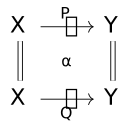
and
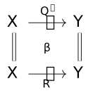
in their theory when Q \neq Q'. The system must therefore be able to detect when a theory is invalid. As our objective is to eliminate undesirable runtime behaviors, a reasonable angle of attack would be to look for a type theory that reflects the structure of double categories, and rejects illegal moves like the ones described above.
Although we have only spoken of double categories so far, we are principally interested in virtual double categories (VDCs) [1,2,5]. These generalize double categories by weakening the categorical structure of the loose direction, dropping the requirement that proarrows have composites or identities. Virtual cells have a proarrow domain of a sequence of “composable” proarrows (meaning the target object of one proarrow is the source of the next), and can only be tightly composed. Because composites of virtual cells organize themselves into tree-like structures, they are more amenable to a computer representation—in an ordinary double category, one can end up with arbitrarily complex pasting diagrams of cells composed along both the tight and loose directions, but in a VDC we can only combine cells from top to bottom. Because of their directed cells, VDCs also enjoy a more “unbiased” composition than ordinary double categories, by excluding pinwheel-like pasting diagrams.
1 A Type Theory for VDCs
Our approach was inspired by Hayato Nasu’s prior work on a type theory for the internal language of (cartesian, fibrational) VDCs [6], and shares a similar syntax and vocabulary. Since our objective is to implement a (decidable) corresponding typechecking procedure in a programming language we give special attention to matters of computability and normalization; indeed, part of the appeal of Nasu’s thesis was its uniform treatment of cell restriction.
The type theory is stratified into two levels of typing judgment,2 corresponding to the two strata of a virtual double category:
objects correspond to types and tight morphisms to terms.
proarrows are viewed as “protypes,” which are assigned to “proterms” representing virtual cells.
This approach of viewing objects as types and morphisms as terms is standard in categorical logic [7]. A common theme in double category theory is that the proarrows of a VDC are a kind of morphism that also behave like objects; that is, they can be thought of as objects that happen to have a source and target, and hence correspond to a kind of binary dependent type. Cells from a sequence of proarrows to some other proarrow then look like multiary morphisms between these dependent types—we think of a virtual cell
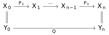
as a kind of n-ary function with arguments of “types” P_1, \dots, P_n and output “type” Q.
The formal judgments of this type theory are summarized below:
| Judgment | Notation |
|---|---|
| \mathrm{Type} | X \text{ type} |
| \mathrm{Context} | \Gamma \text{ ctx} |
| \mathrm{Term} | \Gamma \vdash s : X |
| \mathrm{Protype} | \Gamma_0 , \Gamma_1 \vdash \underline{P} \text{ protype} |
| \mathrm{Boundary} | \Gamma_0, \dots, \Gamma_n \mid \underline{P}_1, \dots, \underline{P}_n \to \underline{Q} |
| \mathrm{Procontext} | \Gamma_0, \dots, \Gamma_n \mid p_1 : \underline{P}_1, \dots, p_n : \underline{P}_n \text{ proctx} |
| \mathrm{Proterm} | \Gamma_0, \dots, \Gamma_n \mid p_1 : \underline{P}_1, \dots, p_n : \underline{P}_n \vdash \tau : \underline{P} |
We will often denote a sequence of (unary) term contexts \Gamma_0, \dots, \Gamma_1 by \overline{\Gamma}, and we will abbreviate a sequence of proterm bindings p_1 : \underline{P}_1, \dots, p_n : \underline{P}_n by \Omega.
The first three judgments, which specify the type theory for the object and tight morphism level, are simply the unary type theory for a category as described in [7]. We will review what this means, but most of our attention will be focused on the last four judgments, which define the type theory for the proarrow and cell level. For brevity we elide the full BNF of the language’s constructs; most of the grammar can (I hope) be easily inferred from the typing judgments.
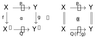
Since the VDCs we are interested in are fibrational (i.e. have restrictions), we are safe to assume all of our cells are globular; we identify cells with nontrivial tight morphisms (like the cell on the left) with the induced globular cell into their codomain’s restriction (the cell on the right):
1.1 Signature
The type theory for a particular virtual double theory \mathbb{T}_\Sigma is parameterized by a signature \Sigma, which should be thought of as akin to the signature of an algebraic theory, consisting of
a set3 of object symbols \mathcal{T}_\Sigma.
a set of function symbols \mathcal{F}_\Sigma(X, Y) for each pair X, Y \in \mathcal{T}_\Sigma.
a set of proarrow symbols \mathcal{P}_\Sigma(X, Y) for each pair X, Y \in \mathcal{T}_\Sigma.
a set of cell symbols \mathcal{C}_\Sigma, each of which is associated with a boundary specifying its arity, domain, and codomain.
The exact nature of the boundaries of the cell symbols in \mathcal{C}_\Sigma requires that we first introduce the foundation of the type theory. Namely, in order to make sense of the shapes of cells, we must understand terms and protypes, so we will make (4) formal in Section 1.3 after we have built up the necessary technology.
1.2 Types, Terms, and Pointful Syntax
The type theory in the tight direction is simple and not particularly interesting. Types are simply the category symbols X \in \mathcal{T}_\Sigma, while terms are typed in a unary context \Gamma = (x : X) consisting of exactly one variable binding. The typing judgments for terms are typical for a unary 1-categorical type theory [7]:

We pause to emphasize the pointful nature of this syntax, in contradistinction to the point-free syntax we are accustomed to in category theory. For instance, given morphisms \begin{aligned} f &: X \to Y\\ g &: Y \to Z\\ h &: Z \to W \end{aligned} in the usual point-free syntax we can express their composite in two equivalent ways: h \circ (g \circ f) = (h \circ g) \circ f. However, if we were to express this composite “pointfully,” say in a context x : X, we could only write x : X \vdash h(g(f(x))) : W. Similarly, the identity morphism \operatorname{id}_X : X \to X can be expressed pointfully as simply x : X \vdash x : X, so the equivalent point-free composites f = \operatorname{id}_Y \circ f = f \circ \operatorname{id}_X = \operatorname{id}_Y \circ \operatorname{id}_Y \circ f \circ \operatorname{id}_X \circ \operatorname{id}_X all have the unique form x : X \vdash f(x) : Y. (This, of course, requires some notion of a signature in the same sense as above to make sense, otherwise expressions such as x : X \vdash \operatorname{id}_X(x) : X would be just as valid.)
It is not hard to see why having a canonical presentation like this might be desirable, since it eliminates the need to explicitly select a paranthesization and quotient the syntax by its underlying semantics. The contrast between pointful and point-free syntax is discussed more thoroughly in [8].
1.3 Protypes and Procontexts
We are now equipped with the necessary background to study the more interesting component of the type theory, which describes the proarrows and cells of \mathbb{T}_\Sigma; the former are represented by protypes (types in the “pro” direction), and the latter by proterms (which are typed in ordered procontexts), discussed in Section 1.4.
Protypes depend on a pair of (unary) term contexts (\Gamma_0, \Gamma_1), which can be thought of as its domain and codomain (respectively). Every proarrow symbol P \in \mathcal{P}_\Sigma gives rise to a dependent family of protypes, which are parameterized by a pair of suitably-typed terms:

When s and t are not relevant we denote a protype simply by \underline{P} = P(s, t) for brevity.
Viewing the terms s, t as tight morphisms and P as a proarrow X \mathrel{\mkern 3mu\vcenter{\hbox{$\shortmid$}}\mkern-10mu{\to}}Y, the protype P(s, t) represents the restriction of P along s and t, which is itself a proarrow from the type of \Gamma_0 to the type of \Gamma_1. This captures the fibrational structure of \mathbb{T}_\Sigma.
We can at last fulfill our vow from Section 1.1 to revisit the boundaries of the signature’s cell symbols. Each cell symbol \alpha \in \mathcal{C}_\Sigma is associated with a boundary declaration of the form

We say that \alpha has arity n, with (proarrow) domain \underline{P}_1, \dots, \underline{P}_n and (proarrow) codomain \underline{Q}. This can be thought of as an n-ary function “into” \underline{Q}, taking as “input” other cells mapping “into” \underline{P}_1, \dots, \underline{P}_n. From the perspective of dependent type theory, one can view \alpha as a term of a particular dependent function type \alpha : \textstyle \prod_{x_j : X_j} \prod_{p_i : \underline{P}_i} \underline{Q}, where \underline{P}_i depends on x_{i-1} and x_i, and \underline{Q} depends on x_0 and x_n.
In Section 1.4 we make the analogy with n-ary functions precise with the (pro)typing judgments for proterms. Procontexts, the contexts for these judgments, consist of precisely the data of the domain of a virtual cell—namely, a sequence of n + 1 types X_0, \dots, X_n, and a sequence of protypes \underline{P}_1, \dots, \underline{P}_n with \underline{P}_i typed by x_{i-1}:X_{i-1}, x_i : X_i. Explicitly:

We denote a procontext \Gamma_0, \dots, \Gamma_n \mid p_1 : \underline{P}_1, \dots, p_n : \underline{P}_n by \overline{\Gamma} \mid \Omega.
The ordering on \Omega is essential, and the resulting type theory on proterms bears a close resemblance to an ordered linear logic [9,10]. This corresponds to the fixed order of the proarrows in the domain of a cell. When typing a proterm in procontext \overline{\Gamma} \mid p_1 : \underline{P}_1, \dots, p_n : \underline{P}_n, every proterm variable p_1, \dots, p_n must be consumed in sequence, and cannot be used more than once. One consequence of this ordering, and the requirement that the domain term context of each protype in \Omega agrees with the codomain term context of its predecessor, is that we must take special care when concatenating a pair of procontexts. We define a partial function \vee, the join \overline{\Gamma} \vee \overline{\Gamma}' of (nonempty) term context sequences, by (\overline{\Gamma}_L, x : X) \vee (x : X, \overline{\Gamma}_R) := \overline{\Gamma}_L, x : X, \overline{\Gamma}_R and is otherwise undefined when \overline{\Gamma} does not end with the same term context that \overline{\Gamma}' begins with. (Whenever the join of two or more term context sequences appears in the consequent of a formal judgment, there is an implicit hypothesis that it is defined.)
1.4 Proterms
Modulo their ordered contexts, the basic typing judgments for proterms appears similar to the (cut-free) type theory for multicategories [7], with a rule for introducing (proterm) variables providing the leaf nodes of a derivation tree and a rule for applying cells given by the signature supplying the internal nodes. The former is straightforward:

and the omission of any extra term or proterm data in the procontext enforces its linearity. The cell application rule is slightly more subtle; a first attempt, which is essentially the rule given in [6], might look something like

(Here t[s/x] indicates the substitution of s for x in t, defined in the usual way. We discuss both term and proterm substitutions in more detail in Section 2.1.) Note that the domain of the cell symbol \alpha in this rule contains only term variables, but no real terms.
This works for the slightly more restrictive case where we only want to permit proarrows in the signature to appear in the domain of a cell. The type theory presented in [6] makes this assumption, in which case the rule above suffices, but we aim to generalize to the setting where primitive cells can have restrictions in their domain (see Example 3.2.2 for a virtual double theory that requires cells of this form), such as
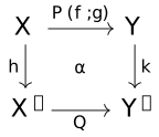
Here the cell \alpha would have signature \alpha : (x : X, y : Y \mid P(f(x), g(y))) \to Q(h(x), k(y)) which is not compatible with our candidate rule for cell application.
The problem is that, given some other cell
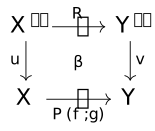
we cannot form the composite of \alpha with \beta with the typing judgment above, because \beta is typed via a derivation of the form x'' : X'', y'' : Y'' \mid r : R(x'', y'') \vdash \beta(r) : P(f(u(x'')), g(v(y''))), while \alpha expects a proterm with protype P(f(x), g(y)). The typing rule for composition with \alpha must therefore have some mechanism for unifying x with u(x'') and y with v(y''). We achieve this by allowing the protype of the cell’s arguments to “specialize” (more precisely, to be restrictions of) the expected protypes. This is almost suggestive of a form of subtyping relation on protypes, witnessed by restrictions; a cell \alpha expecting an input of protype P(f(x), g(y)) can be passed an argument of protype P(f(h(x')), g(k(y'))), for example.
There is another subtlety that the rule above sweeps under the rug, pertaining to nullary cells (i.e. cells with an empty proarrow domain). With our naïve syntax for cell application, there is no way to disambiguate the cells below
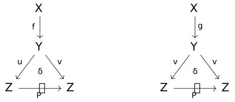
since both would be expressed as \delta() in our grammar. One option would be to introduce a separate typing judgment with a special term annotation for nullary proterms, but this feels inelegant4 and somewhat artificial. Instead, we prefer to make our syntax slightly more verbose by annotating every n-ary cell application with its n+1 term arguments5; the unary cell \alpha defined above is expressed as the proterm x : X, y : Y \mid p : P(f(x), g(y)) \vdash \alpha\{x, y\}(p) : Q(h(x), k(y)), and we can distinguish the previous pair of nullary cells via the proterms x : X \mid \cdot \vdash \delta\{f(x)\}() : P(u(f(x)), v(f(x))) and x : X \mid \cdot \vdash \delta\{g(x)\}() : P(u(g(x)), v(g(x))). Going forward we will typically omit empty proterm arguments, simply writing \delta\{f(x)\} for the first of these nullary cells, for example.
In light of the extensions above, we adapt our first attempt at the typing judgment for cell application into the slightly more intimidating

Here, and in the sequel, \underline{P}\langle s, t \rangle abbreviates substituting the term s for the left term variable and t for the right term variable in \underline{P}. For example, we could have instead written \underline{P}_i[s_{i-1}/x_{i-1}, s_i/x_i] and \underline{Q}[s_0/x_0, s_n/x_n] above instead.
(The ugly whiskering of the term context’s join by y_0 and y_n is another annoying consequence of accomodating nullary cells. When n = 0 the sequents degenerate into a single term judgment y_0 : Y_0 \vdash s_0 : X_0 and no proterm judgments, so we must ensure that y_0 : Y_0 makes it into the antecedent’s context. In this case whiskering by y_n : Y_n on the right is redundant, the y_0 on the left suffices; we only include it for aesthetic reasons, and so that it doesn’t feel left out.)
1.5 Examples
The best way to understand this type theory is through exposure, so we will wrap up this section with a few self-contained examples. These take for granted the correspondence between proterms and cells in a VDC, which we make formal in Section 2.
The simplest example of a cell, the identity cell on a proarrow P is represented by a proterm variable, in the same sense that a term x : X \vdash x : X represents the morphism \operatorname{id}_X in the (unary) type theory of categories [7]. Concretely, we would denote the identity cell
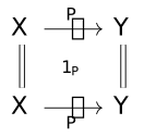
using the procontext and proterm x : X, y : Y \mid p : P(x, y) \vdash p : P(x, y). Note that the names of the term variables x, y and proterm variable p were chosen arbitrarily (i.e. proterms should only be considered up to \alpha-equivalence).
Next, we consider a single (binary) cell
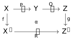
which we assume to belong to our signature with the appropriate sort—that is, \alpha \in \mathcal{C}_\Sigma has boundary (x : X, y : Y, z : Z \mid P(x, y), Q(y, z)) \to R(f(x), g(z)). To express this cell as a proterm, we would write \begin{aligned} &x : X, y : Y, z : Z \mid p : P(x, y), q : Q(y, z) \\ &\hspace{0.6em}\vdash \alpha\{x, y, z\}(p, q) : R(f(x), g(z)). \end{aligned}
Suppose we extend Example 2 by precomposing with cells \beta and \gamma (again, cell symbols in \mathcal{C}_\Sigma with the appropriate boundaries), as below:
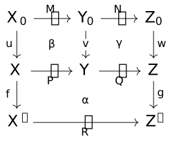
This composite cell is represented by the proterm \begin{aligned} &x : X_0, y : Y_0, z : Z_0 \mid m : M(x, y), n : N(y, z) \\ &\hspace{0.6em}\vdash\alpha\{u(x), v(y), w(z)\}(\beta\{x, y\}(m), \gamma\{y, z\}(n)) : R(f(u(x)), g(w(z))). \end{aligned}
For our final example, we’ll look at how restriction can be expressed in the language of proterms. Given a proarrow P, the restriction cell itself has the form
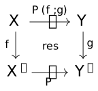
so the corresponding proterm \tau, whatever it may be, must fit into a typing judgment of the form x : X, y : Y \mid p : P(f(x), g(y)) \vdash \tau : P(f(x), g(y)). But the variable p in the procontext has exactly the expected type, so in fact both the identity cell on P(f;g) and the restriction cell for P along f and g are represented by the same proterm p.
Similarly, a cell
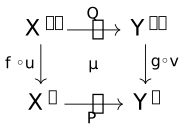
represented by x : X'', y : Y'' \mid q : Q(x, y) \vdash \mu\{x, y\}(q) : P(f(u(x)), g(v(y))), induces a cell
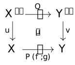
via the universal property of restriction. Writing \rho for the corresponding proterm, we should have a typing judgment of the form x : X'', y : Y'' \mid q : Q(x, y) \vdash \rho : P(f(u(x)), v(g(y))) Again, this is matches the judgment for the original cell \mu. The syntax of proterms exactly captures the universal property of restriction by identifying a cell with its restrictions. If we were to consider the induced cell into P(f\circ u; g \circ v), we would again find that it is represented by the proterm \mu\{x, y\}(q) in the same procontext, and with the same protype.
2 Semantics
So far we have presented a type theory that ostensibly reflects the internal logic of a virtual double theory. However, for this syntax to be meaningful, it must be equipped with a suitable semantics which realizes the structure of a VDC. The examples of Section 1.5 hint at the expected behavior of this VDC. In this section we establish an interpretation \llbracket \Sigma \rrbracket of a particular signature \Sigma as a free VDC, allowing us to recover the theory’s interface from its syntactic presentation.
To make sense of this, we need to take a brief detour into substitutions, which until now we have mostly taken for granted.
2.1 Substitution
Substitution holds a special place in type theory, analogous to composition in category theory. (In some sense this is more than just an analogy, since in the categorical semantics of a type theory one frequently realizes composition via substitution.) We have already seen how we need to make use of substitution in our cell application typing judgment, to facilitate non-globular cells.
So far we have left the mechanics of substitution implicit. Indeed, term substitution holds no nasty surprises. These substitutions benefit from the property of cut elimination [7], which says that substitution is admissible (informally, that it behaves well with respect to the type theory for terms and does not require its own typing judgment). The slogan to have in mind is “any term of type X can be used in place of a variable of type X.” Similarly, substitution plays nicely with protypes (which is not surprising given that a protype is effectively just a wrapper for a pair of terms labeled by some element of \mathcal{P}_\Sigma):
This lemma allows us to “precompose” by a pair of terms, lifting the context of a protype. This sounds similar to restricting a proarrow by a pair of tight morphisms in a fibrational VDC, and in fact it is precisely through this substitution property for protypes that we will recover fibrationality in the VDC semantics of our type theory in Section 2.2.
Similarly, we can substitute suitably typed terms for term variables inside of a proterm, pulling the context back. Note that because these term variables may appear in the procontext, this substitution occurs not only within the proterm itself, but also in every protype in sight (both the protype of the term and the protypes in the procontext).
Again, we will see in Section 2.2 that the substitution \tau [\overline{s_i/x_i}] corresponds semantically to restriction along s_0, \dots, s_n.
We likewise have a notion of proterm substitution, whereby we replace a proterm variable with some other proterm with a compatible type. This is slightly more subtle than ordinary term substitution, because we also need to substitute for the term variables present in both the proterm and its procontext (as we did in Lemma 2).
It is essential that we be able to substitute (say) \tau : P(f(x), g(y)) for a variable p : P(x', y') to make sense of tight cell composition, but in order for this substitution to be sound it must ablate all occurances of x' and y' in sight, even within the procontext. But the term variables occuring on the boundary of one proterm variable are shared by its neighbors, so we cannot merely perform a single, local proterm substitution. This reflects the signature of cell composition in a VDC, which demands that each proarrow of the domain be supplied with a cell with a matching codomain.
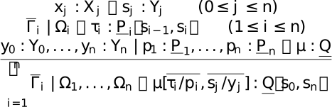
We capture this “wide” substitution operation with the analogous “multi-substitution” rule which, like substitution for terms, is admissible in our type theory:
The multi-substitution rule for proterms
is admissible.
This rule closely resembles the cell application rule of Section 1.4, which supports our intention for proterm substitution to materialize cell composition in the semantics: applying a single, atomic cell \alpha \in \mathcal{C}_\Sigma to appropriately typed \tau_1, \dots, \tau_n should be the same as composing \alpha with each \tau_i.
2.2 The Semantic VDC
Given a signature \Sigma as defined in Section 1.1, we denote by \llbracket \Sigma \rrbracket the free semantic VDC generated by \Sigma, where \llbracket \Sigma \rrbracket has
an object \llbracket X \rrbracket for each type X,
a (tight) morphism \llbracket s \rrbracket : \llbracket X \rrbracket \to \llbracket Y \rrbracket for each term x : X \vdash s : Y,
a proarrow \llbracket \underline{P} \rrbracket : \llbracket X \rrbracket \mathrel{\mkern 3mu\vcenter{\hbox{$\shortmid$}}\mkern-10mu{\to}}\llbracket Y \rrbracket for each x : X, y : Y \vdash \underline{P} \text{ protype},
and a cell
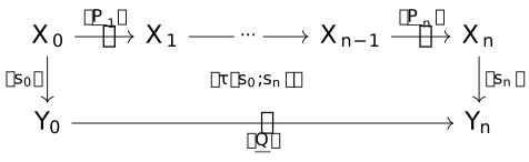
for each pair of terms X_i \vdash s_i : Y_i for i = 0, n and proterm x_0 : X_0, \dots, x_n : X_n \mid p_1 : \underline{P}_1, \dots, \underline{P}_n \vdash \tau : \underline{Q} \langle s_0, s_n \rangle. Terms, protypes, and proterms are only considered up to \alpha-equivalence, so the choice of variable names does not distinguish a pair of otherwise identical morphisms or cells.
The interpretation \llbracket - \rrbracket maps syntax to semantics, making rigorous the correspondence we gestured towards in previous sections. The categorical structure of the tight direction is defined in the expected way [7], whereby term variables are identity morphisms: \operatorname{id}_{\llbracket X \rrbracket} := x : X \vdash x : X and, given x : X \vdash s : Y and y : Y \vdash t : Z, term substitution provides composition: \llbracket t \rrbracket \circ \llbracket s \rrbracket := \llbracket t[s/y] \rrbracket, where x : X \vdash t[s/y] : Z by cut elimination for terms.
On the other hand, the semantics for protypes and proterms is similar to a free multicategory [7]. Unlike the type theory of multicategories, however, cells in \llbracket \Sigma \rrbracket depend not only on a proterm, but are also parameterized by a pair of terms. Note that we cannot omit these terms, since the syntax identifies each cell with the canonical globular cell it induces via restriction; the outer terms disambiguate which of these cells we are referring to. This is consistent with ordinary categories, where the domain and codomain of a morphism are part of its data.
To finish making \llbracket \Sigma \rrbracket into a VDC, for each pasting diagram of the form
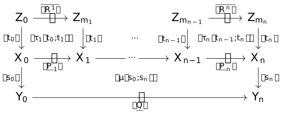
we must specify a (tight) composite cell
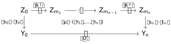
This is supplied by Lemma 3 via the proterm z_0 : Z^0, \dots, z_{m_n} : Z_{m_n} \mid \Omega_1, \dots, \Omega_n \vdash \mu[\overline{\tau_i/p_i}, \overline{t_j/z_j}] : \underline{Q}\langle s_0[t_0/x_0], s_n[t_n/x_n] \rangle along with the terms z_0 : Z_0 \vdash s_0[t_0/x_0] : Y_0 and z_{m_n} : Z_{m_n} \vdash s_n[t_{m_n}/x_n]. Multi-substitution elimination (Lemma 3) guarantees that this proterm is well-typed and the corresponding cell in \llbracket \Sigma \rrbracket has the correct boundary.
Finally, if we want our VDC to be fibrational, we need to define restrictions. Given a proarrow \llbracket \underline{P} \rrbracket and morphisms \llbracket s \rrbracket and \llbracket t \rrbracket as below, we construct the restriction proarrow and cartesian cell
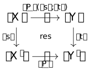
as follows: since \llbracket \underline{P} \rrbracket : \llbracket X' \rrbracket \mathrel{\mkern 3mu\vcenter{\hbox{$\shortmid$}}\mkern-10mu{\to}}\llbracket Y' \rrbracket, we have a judgment of the form x' : X', y' : Y' \vdash \underline{P} \text{ protype}. Similarly, we have judgments \begin{aligned} x : X &\vdash s : X'\\ y : Y &\vdash t : Y' \end{aligned} so it follows from Lemma 1 that x : X, y : Y \vdash \underline{P}\langle s, t \rangle \text{ protype}, which represents the cartesian proarrow \llbracket \underline{P} \rrbracket (\llbracket s \rrbracket ; \llbracket t \rrbracket ) : \llbracket X \rrbracket \to \llbracket Y \rrbracket. The cartesian cell \mathrm{res} is represented by the proterm x : X, y : Y \mid p : \underline{P}\langle s, t\rangle \vdash p : \underline{P}\langle s, t\rangle together with the terms x : X \vdash s : X' and y : Y \vdash t : Y'.
Why do the proarrow and cell defined above satisfy the universal property of the restriction cell? At a high level, the point is that restriction and composition are both defined in terms of substitutions, which can be decomposed. Concretely, suppose given a cell
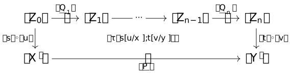
represented by a proterm z_0 : Z_0, \dots, z_n : Z_n \mid q_1 : \underline{Q}_1, \dots, q_n : \underline{Q}_n \vdash \tau : \underline{P}\langle s [u / x], t [v / y] \rangle and the terms s[u/x], t[v/y], where \begin{aligned} z_0 : Z_0 &\vdash u : X\\ z_n : Z_n &\vdash v : Y. \end{aligned} Since \underline{P}\langle s[u/x], t[v/y] \rangle = (\underline{P}\langle s, t\rangle)\langle u, v \rangle, \tau, together with the terms u, v, also represents a cell
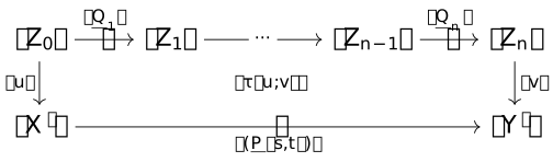
whose proarrow codomain is precisely the restriction proarrow \llbracket \underline{P} \rrbracket (\llbracket s \rrbracket; \llbracket t \rrbracket) defined above. The tight composite of this cell with the cell \mathrm{res} is represented by the proterm p[\tau/p] = \tau and the terms s[u/x], t[v/y], which is exactly the data of the cell we began with. We get uniqueness for free since \tau = p[\tau/p] = p[\tau'/p] = \tau'.
We summarize the discussion above with the following:
Note that both flavors of substitution described in Section 2.1 played a crucial role in defining the semantic VDC \llbracket \Sigma \rrbracket: cell composition manifests itself as proterm substitution, while restriction is obtained from term substitution.
3 A DSL for Virtual Double Theories
A core objective of this project is to produce a DSL providing advanced users or developers of CatColab with an interface into the virtual double theories it uses to structure data. While a finalized version of this language is still under development, the current prototype closely follows the basic syntax of Section 1, and supports bidirectional (pro)typechecking to validate the specification of a theory.
This is particularly relevant to verifying the axioms of a virtual double theory. Although we have primarily focused on VDCs freely specified by a given signature, most interesting virtual double theories are quotients of free semantic VDCs by some given equalities. While we will not discuss the denotational semantics underlying these VDCs in this post, the idea is that we would like to impose some relationships on the morphisms or cells of the virtual double theory that capture the desired behavior of its models. The main purpose of type-checking in the DSL is to ensure that the composites of cells appearing in these axioms are well-formed, and that a pair of cells identified by an axiom have compatible boundaries.
3.1 Surface Syntax
The user-facing language for the DSL is intended to be relatively straightforward to learn and use. To that end, we aim to minimize the amount of annotations and explicit indexing exposed in the surface syntax, and infer as much data as possible when passing to the intermediate representation. For instance, the term arguments to a non-nullary cell application can always be deduced from the protypes of its one or more proterm argument(s); in the nullary case a single term argument annotation is still necessary, for the reasons discussed previously.
To declare the signature \Sigma of a theory, the user specifies object symbols with statements like the following:
obj X       -- declares an object symbol X
obj [Y, Z]  -- declares object symbols Y, Z
Similarly, function symbols \mathcal{F}_\Sigma and proarrow symbols \mathcal{P}_\Sigma can be added to the signature by specifying their domain and codomain:
-- function symbol declarations
fun f : X -> Y
fun g : Y -> Z

-- proarrow symbol declarations
pro P : X => Y
pro Q : Y => Z
pro R : X => Z
The syntax for the cell symbols \mathcal{C}_\Sigma closely resemble the boundary declarations of Section 1.3:
-- declares a unary cell α from P to Q with source
-- arrow f and target arrow g
cell α : [x : X, y : Y] | [P[x, y]] -> Q[f(x), g(y)]

-- declares a globular binary cell β from [P, R] to Q
cell β : [x : X, y : Y, z : Z] | [P[x, y], Q[y, z]] -> R[x, z]
Many of the theories we are interested in require one or more (strict) equalities between proarrows. For instance, the theory of promonads (Example 3.2.1) has the equality of protypes as an axiom. To preserve syntax-directed typechecking, we forbid this kind of anonymous, proof-irrelevant6 equality, and instead adopt an approach closer to the homotopy type theorist’s path terms. Namely, transport between protypes that are intended to be “equal” is handled by a special cell isomorphism declaration:
-- provides an isomorphism between the proarrows P(g; id) and Q(id; g)
iso [y0 : Y, y1 : Y] ⊢ [p2q, q2p] : P[g(y0), y1] <=> Q(y0, g(y1))
Protype isomorphisms can be used like any other cell symbol (note that they are always unary), allowing any proterm whose protype lives on one side of the isomorphism to be used as a proterm belonging to the other protype. By making the application of an isomorphism explicit, we can use the existing typechecking procedure without needing any extra infrastructure to accomodate non-syntactic equalities.
Lastly, axioms impose additional equalities on proterms. These expressed with a similar syntax to cell declarations:
-- declares a proterm axiom making a globular cell γ : P => P idempotent
axiom [x : X, y : Y] | [p : P[x, y]] ⊢ γ [γ [p]] ≡ γ [p]
Every protype isomorphism implicitly adds a pair of axioms witnessing that the two cell symbols are inverses. For instance, under the hood the isomorphism declaration above would introduce the following axioms:
axiom [y0 : Y, y1 : Y] | [_p0 : P[g(y0), y1]] ⊢ q2p[p2q[_p0]] ≡ _p0
axiom [y0 : Y, y1 : Y] | [_p1 : Q[y0, g(y1)]] ⊢ p2q[q2p[_p1]] ≡ _p1
The language’s syntax, at least in its current form, was heavily influenced by Owen Lynch’s fnotation, which saved me countless hours that would otherwise have been spent writing frontends for the various iterations of this project. Thanks Owen!
3.2 Examples
The theory of promonads consists of a single object X, a proarrow P : X \mathrel{\mkern 3mu\vcenter{\hbox{$\shortmid$}}\mkern-10mu{\to}}X, and a globular nullary cell
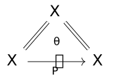
subject to the following axioms:
P = P \odot P
there are equalities of cells
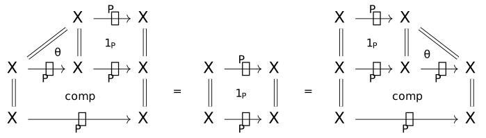
We have (very deliberately) tiptoed around loose composition, for reasons discussed in Section 4. For the purposes of this example, we manually declare a composite cell with the required boundary, allowing us to express this theory as follows:
obj X
pro P : X => X
cell θ : [x : X] -> P[x, x]
cell comp : [x0 : X, x1 : X, x2 : X | P[x0, x1], P[x1, x2]] -> P[x0, x2]

axiom [x0 : X, x1 : X] | [p : P[x0, x1]] ⊢ comp[θ(x0), p] ≡ p
axiom [x0 : X, x1 : X] | [p : P[x0, x1]] ⊢ comp[p, θ(x1)] ≡ pThere are several ways to present the theory of adjunctions f : X \leftrightarrows Y : g, corresponding to the many equivalent definitions of an adjunction. Any such presentation will contain objects X and Y, together with morphisms f : X \to Y and g : Y \to X:
obj [X, Y]
fun f : X -> Y
fun g : Y -> X
We will also need to use the loose units on X and Y, which we define manually by
pro idX : X => X
pro idY : Y => Y
because we have not talked about how to incorporate these into our type theory (see Section 4).
One option to present the axioms of this theory is a pair of inverse cells, which witness the natural isomorphism of hom-sets (which are represented by the unit proarrows):
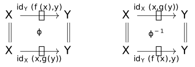
We can write this in our DSL as
-- inverse cells
cell l2r : [x : X, y : Y] | [l : idY[f(x), y]] -> idX[x, g(y)]
cell r2l : [x : X, y : Y] | [r : idX[x, g(y)]] -> idY[f(x), y]

-- axioms making the cells inverses
axiom [x : X, y : Y] | [l : idY[f(x), y]] ⊢ r2l[l2r[l]] ≡ l
axiom [x : X, y : Y] | [r : idX[x, g(y)]] ⊢ l2r[r2l[r]] ≡ r
or more succinctly as
-- simultaneously declares the cells l2r and r2l along with the axioms making them inverses
iso  [x : X, y : Y] ⊢ [l2r, r2l] : idY[f(x), y] <=> idX[x, g(y)]
This particular presentation of the theory of adjunctions highlights why we need to allow cells to map out of restricted proarrows, which is the “wrong” direction relative to the universal property. We can always pull terms (i.e. tight morphisms) into or out of the codomain, but any terms in the domain of a cell cannot be extracted.
4 Future Work
The basic type theory outlined above—which generalizes Nasu’s prior work [6] by facilitating a broader range of primitive cells through our slightly more expressive composition rule—has remained more or less fixed throughout each iteration of this project. However, there are many important extensions to the language presented in this post that I am still working on understanding, and finding the right way to set up the type theory so that the underlying categorical semantics are preserved while maintaining an acceptable degree of computability has been a serious challenge. We’ll wrap up with a summary of the many loose ends that have been keeping me up at night.
In practice, we often wish to make use of additional structure in a virtual double theory. For instance, recall that in Example 3.2.1 we needed to define loose composition by hand, and similarly in Example 3.2.2 we had to manually declare loose units. Ideally, we would like our type theory and DSL to support loose units and composites natively, but this turns out to be a surprisingly subtle issue.
In [6], loose units are treated as a kind of directed path type, similar to the identity type of homotopy type theory. The universal nullary cell along a given morphism into the loose unit is realized as a kind of reflexive path, and the universal property resembles path induction. Unfortunately, there are some technical obstructions to directly adapting this approach for our use case. The main issue is finding some normalization procedure so that, for instance, one can compute that the following three cells are equivalent:
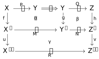
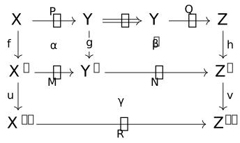
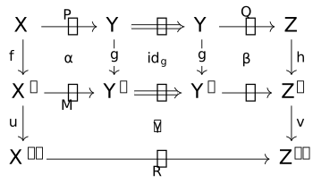
(where \widetilde{\alpha}, \widetilde{\beta}, and \widetilde{\gamma} denote the cells induced by the universal property of the loose unit).
I have spent a lot of time trying to find the right operational semantics to capture the universal property of units as directed reduction rules, with equivalent cells being expressed by proterms which evaluate to a common normal form. This may seem non-obvious, since up to this point our language has been essentially static, and a priori there is no reason to expect such a normalization procedure to exist. The point is that universal properties are often expressed via computation rules (i.e. \beta and \eta reduction) in type theory, and indeed this is the approach taken in [6]. However, requiring that proterms be both expanded and reduced to establish an equivalence is unlikely to be computable; we aim to endow these rules with a directionality, so that universal properties are expressed by reducing proterms until they are fully “evaluated”.
Another recurring issue in attempting to integrate loose units into our language has been their tight coupling with loose composites. This is not addressed in [6], but for our purposes understanding the interactions between units and composites is crucial. Like with units, we also aim to capture the universal property of composites using the language’s operational semantics. Finding the right reduction rules to make all of this work, while also correctly handling the interactions between units and composites, is subtle, and I have not yet found the right way to do this.
Since the start of this project I have also planned on supporting virtual double theories with modalities; that is, equipped with a double monad that commutes with all visible structures (one should imagine the list monad). These are necessary to define, for instance, an unbiased theory of monoidal categories.
It is not difficult to integrate modalities into the syntax or type theory. In fact, this is fairly straightforward by simply taking the closure of the existing generators under application of the specified monad(s). The challenge lies primarily in the monad axioms. The axioms on cells are no different from the axioms our DSL already supports, but the equalities on tight morphisms complicate the typechecking procedure. I have played around with using e-graphs [11,12] to handle equalities at the morphism level, but this feels somewhat inelegant (in some sense the entire purpose of this project is to avoid relying on such tools) so I am hoping to find a cleaner solution to this problem.
Finally, recall that we only covered the denotational semantics for the free semantic VDC \llbracket \Sigma\rrbracket generated by the signature, without any mention of the cell axioms used by the DSL. These axioms are what give form to the virtual theories we are interested in, so an honest accounting of the type system governing our language should have semantics that capture the quotient of \llbracket \Sigma \rrbracket by these equalities. One of the auxiliary objectives of this project is to get a better handle on the notion of a (finite) presentation of a VDC by generators and relations, which is currently not well understood.
5 References
Footnotes
To be precise, a model for a double theory \mathbb{T} in \mathbb{S} is a double functor \mathbb{T} \to \mathbb{S} respecting some additional structure; see [2].↩︎
These are analogous to the two categories D_1 \rightrightarrows D_0 of a double category, as an internal category in \mathrm{Cat}.↩︎
We are being slightly imprecise here. In general one should take more care with size-related issues, but since we are interested in representing our theories in a computer the data of \Sigma will not only be a set, but in fact will be a finite.↩︎
Although frankly the mangled typing judgment we’ll end up with is not much prettier.↩︎
Our surface syntax can infer these term arguments for n > 0, so our DSL only requires them in the nullary case. In this way we spare users from paying the price for our type-theoretic sins as much as possible.↩︎
In the sense that any two equalities are considered identical.↩︎